5 Databases and dplyr
5.1 Intro to connections
Use connections to open open a database connection
Load the
connectionspackageUse
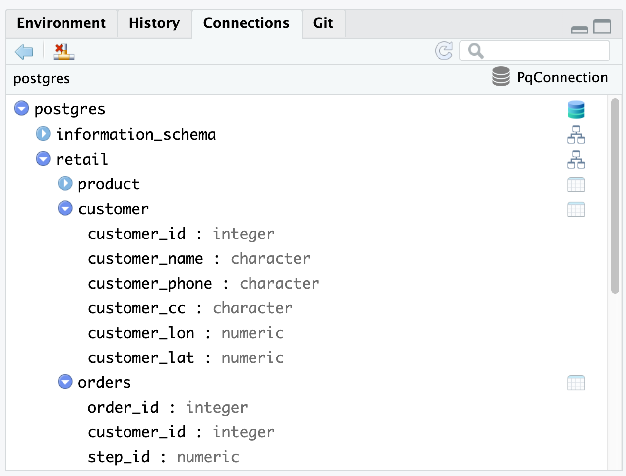
connection_open()to open a Database connectionThe RStudio Connections pane should show the tables in the database
5.2 Table reference
Use the dplyr’s tbl() command
Load the
dplyrpackageAdd
in_schema()as an argument totbl()to specify the schema## # Source: table<retail.customer> [?? x 6] ## # Database: postgres [rstudio_admin@localhost:5432/postgres] ## customer_id customer_name customer_phone customer_cc customer_lon customer_lat ## <int> <chr> <chr> <chr> <dbl> <dbl> ## 1 1 Marilou Donne… 046-995-9387x… 4054106117… -122. 37.8 ## 2 2 Aubrey Gulgow… (020)136-2064 6759766520… -122. 37.7 ## 3 3 Arlis Koss 145.574.8189 8699968904… -122. 37.8 ## 4 4 Duwayne Walsh 737-897-1968x… 4091991124… -122. 37.7 ## 5 5 Nehemiah Doyl… (035)642-3662… 3709535249… -122. 37.7 ## 6 6 Meggan Bruen 326-151-4331 4964180480… -122. 37.7 ## 7 7 Tracie Swift … 776.442.3270x… 4354911637… -122. 37.8 ## 8 8 Karrie Donnel… 883.024.5322x… 4232403376… -122. 37.8 ## 9 9 Kip Eichmann (619)169-8761… 5177848238… -122. 37.7 ## 10 10 Ms. Ciarra Bo… 964-240-3124 4893126879… -122. 37.8 ## # … with more rowsLoad the results from the
tbl()command that points the table called orders to a variable calledordersUse the
classfunction to determine the object type oforders## [1] "tbl_conn" "tbl_PqConnection" "tbl_dbi" "tbl_sql" ## [5] "tbl_lazy" "tbl"
5.3 Under the hood
Use show_query() to preview the SQL statement that will be sent to the database
Use
show_query()to preview SQL statement that actually runs when we runordersas a command## <SQL> ## SELECT * ## FROM retail.ordersWhen executed,
ordersreturns the first 1000 rows of the remote orders table## # Source: table<retail.orders> [?? x 3] ## # Database: postgres [rstudio_admin@localhost:5432/postgres] ## order_id customer_id step_id ## <int> <int> <dbl> ## 1 801473 58 796 ## 2 801474 19 796 ## 3 801475 4 796 ## 4 801476 10 796 ## 5 801477 81 796 ## 6 801478 89 796 ## 7 801479 56 796 ## 8 801480 53 796 ## 9 801481 70 796 ## 10 801482 37 796 ## # … with more rowsFull results of a remote query can be brought into R with
collectEasily view the resulting query by adding
show_query()in another piped command## <SQL> ## SELECT * ## FROM retail.ordersInsert
head()in between the two statements to see how the SQL changes## <SQL> ## SELECT * ## FROM retail.orders ## LIMIT 6Queries can be assigned to variables. Create a variable called
orders_headthat contains the previous query## <SQL> ## SELECT * ## FROM retail.orders ## LIMIT 6Use
sql_render()andsimulate_mssql()to see how the SQL statement changes from vendor to vendor## <SQL> SELECT TOP(6) * ## FROM retail.ordersUse
explain()to explore the query plan## <SQL> ## SELECT * ## FROM retail.orders ## LIMIT 6 ## ## <PLAN> ## Limit (cost=0.00..0.09 rows=6 width=12) ## -> Seq Scan on orders (cost=0.00..15406.47 rows=1000047 width=12)
5.4 Un-translated R commands
Review of how dbplyr handles R commands that have not been translated into a like-SQL command
Preview how
meanis translated## <SQL> ## SELECT "order_id", "customer_id", "step_id", AVG("order_id") OVER () AS "avg_id" ## FROM retail.ordersPreview how
Sys.Date()is translated## <SQL> ## SELECT "order_id", "customer_id", "step_id", Sys.Date() AS "today" ## FROM retail.ordersUse PostgreSQL native commands, in this case
date## <SQL> ## SELECT "order_id", "customer_id", "step_id", date('now') AS "today" ## FROM retail.ordersRun the
dplyrcode to confirm it works## # Source: lazy query [?? x 4] ## # Database: postgres [rstudio_admin@localhost:5432/postgres] ## order_id customer_id step_id today ## <int> <int> <dbl> <date> ## 1 801473 58 796 2020-01-23 ## 2 801474 19 796 2020-01-23 ## 3 801475 4 796 2020-01-23 ## 4 801476 10 796 2020-01-23 ## 5 801477 81 796 2020-01-23 ## 6 801478 89 796 2020-01-23
5.5 Using bang-bang
Intro on passing unevaluated code to a dplyr verb
Preview how
Sys.Date()is translated when prefixing!!## <SQL> ## SELECT "order_id", "customer_id", "step_id", '2020-01-23' AS "today" ## FROM retail.ordersView resulting table when
Sys.Date()is translated when prefixing!!## # Source: lazy query [?? x 4] ## # Database: postgres [rstudio_admin@localhost:5432/postgres] ## order_id customer_id step_id today ## <int> <int> <dbl> <chr> ## 1 801473 58 796 2020-01-23 ## 2 801474 19 796 2020-01-23 ## 3 801475 4 796 2020-01-23 ## 4 801476 10 796 2020-01-23 ## 5 801477 81 796 2020-01-23 ## 6 801478 89 796 2020-01-23Disconnect from the database using
connection_close